中共高官几次试图招安我成为第三梯队的故事。
这里有很多人还不了解“第三梯队”为何物,我不妨讲述一下中共几次试图招安我成为第三梯队的故事。
我在北大物理系读研期间,中共就几次试图招安我成为他们的“第三梯队”。
1987年,我已经成为北京上上下下众人皆知的“自由化头面人物”。
1987年后,中宣部、公安部每年都会列出百名“自由化头面人物”黑名单,据知情者透露,我每年都是榜上有名,而且是最年轻的头面人物。
1987年,北京举行人大代表选举。我发动北大学生发起精选活动。
我这次订立的目标不是本人参选,而是推出一大群自由化人士参与有组织的团队竞选。
在此之前,北大副校长罗豪才、校办主任黄怀诚就多次找我谈话,苦口婆心第劝我要成为北大的第三梯队重点培养对象。
那时我母亲正在北京广安门医院住院化疗。罗豪才和黄怀诚就几次找我谈话。
罗豪才一见我,就嘘寒问暖,说是否有什么需要校方帮助的,还表示要看视我母亲。
我当即回应:
我母亲生病,是我的私事,也是我的隐私,不关党国大业,无需领导劳心费力。你们是党国要员,有什么大事,不妨直说。
罗豪才和黄怀诚二人就一唱一和地给我拍马屁,说我人才难得,可成大事。说他们非常欣赏我,只要我肯配合,就一定能让我成为第三梯队。
我回应说,我凭啥就不能成为第一梯队,而非得成为的他们的孙子辈的第三梯队啊?
罗豪才耐心地跟我解释,包子要一口一口地吃,相当第一梯队,就得先成为第三梯队。
黄怀诚激将我,“你看看,中央目前选拔重用的第三梯队都是清华的,胡锦涛啊,等等。我们北大人就是不服气,难道我们北大就没人才吗?”
黄怀诚继续激将我:“我都欣赏你就是给人才,将来一定能为我们北大人争光争口气,肯定能被成为优秀的第三梯队。”
我问:“我如何才能成为第三梯队啊?”
黄怀诚立即兴奋地说:“这容易啊,只要我们几个校领导推荐,你就是第三梯队。”
我问:“你们几个就有权推荐第三梯队?你让谁当第三梯队,谁就是第三梯队?”
黄怀诚说:“那当然是啦,北大的校长就有权推荐第三梯队。”
我立即大声说:“我追求的是民主自由,其中就是民主选举。我反对的就是由你们这些当权者来推荐什么第三梯队。”
黄怀诚:“我们不搞西方的那套民主选举,我们实行民主集中制。这是我们的优越性。”
我质疑:“中国的几千年历史反复证明了,如果让你们有权来推荐并决定谁是中国的领导人,我保证你们都会推荐你们自己的儿子、孙子来上位继承权位,中国就会成为世袭制,为了确保这种世袭制,中国就一定是独裁暴政。”
黄怀诚:“你也不能这样门缝里看人,我敢保证,我们北大领导就能做到任人唯贤,不拘一格将人才。”
我问:“既然你们能如此保证,不妨教教我,如何才能成为第三梯队?”
他们见我动心,就高兴地说:“这当然好办,其实,只要你能配合我们工作。”
我说:“你们说清楚点,我该如何配合你们?”
黄淮诚:“这只是要求你平时能跟党组织通通气,不要总是发动上街游行,选举,就是不要总是让中央批评我们北大又带头闹事了。”
我当即答应他们:“既然这样,我也有个条件。你们虽然说了保证培养我,但我还是认为你们会随时说话不算数。”
黄淮诚立即说:“你又什么条件,尽管提。”
我就说:“因为我认为你们肯定会提拔你们自己的子女,我不是你们的子女,你们应该送个千金做抵押,让我也成为你们的女婿干儿子,我才放心。”
黄怀诚笑喷了:“你看你,真会开玩笑。象你这种才子,想找个千金,那还不容易吗?只怕你看不上我们的千金。”
我接着说:“我虽然聪明,但还是没法领会领导的意图。你们要再具体地告诉我该干哪些,不该干哪些,给我制定个行动指南。我保证照办。”
黄淮诚就干脆说:“我们今天扯得太远了。我现在就长话短说,单刀直入,也不兜圈子了,就直接跟你说出我们需要你帮我们做到的几件事。”
接着,黄淮诚就开始跟我详细讨论如何操控北大选举的事。
在此之前的几个月,黄淮诚担任北大选举委员会的负责人,我曾经为了选举人大代表,同黄淮诚有过几次交锋。
最先,我是找到黄怀诚向他请教北大的选举细则,我特别问他我们可以推举哪些人成为代表。黄怀诚当即表示,但凡是中华人民共和国合法公民,都有被选举权。
我当即向他表示,我将推举刚刚被开除党籍的方励之以及中央军委主席邓小平作为海淀区人大代表候选人,我担任这些人的推荐人代表和选民代表。
黄怀诚请示上级给我的答复是我们北大只能推荐我们北大的教职工和学生成为人大代表候选人。我当即同他争论,依照他的选举规则,邓小平就只能占用中南海的人大代表指标,中南海里最多有几千人,却要选出几百个人大代表,这种规则根本就不是共产党实际使用的规则,一定是违宪,也违反党章。
无论我如何理论,黄怀诚就是不准我提名邓小平,也不准我提名方励之。在我的反复逼问下,黄淮诚承诺,只要是北大的教职工或学生,我都能提名,提名后,他保证不再干涉。
我当即同意放弃提名方励之和邓小平,还马上给他递交了一个新的候选人:李淑娴,还包括李淑娴。
看到我妥协了,黄淮诚那个开心啊.
过了几天,黄淮诚才发现,我提名的李淑娴不仅仅是北大物理系副教授,而且更重要的是,她是方励之的太太。那还不是换汤没换药,跟提名方励之是一个味嘛。
黄淮诚那个后悔啊。可是他可是当着很多人跟我担保过的,我还拿到了他的担保书,他也是没法公开反悔。他也知道,如果他反悔,我保证会让他下不了台
黄淮诚虽然不公开反悔,却反复反复地跟我明里暗里过招,就是要将李淑娴的名字从候选人名单中拿下。前几次都是败在我收下了,没拿下来。这次是第四次了。
黄淮诚就直接说:“我们只是要求你在明天的选民代表大会上公开宣布你不再提名李淑娴作为人大代表候选人,只要你做到这一点,就算是配合组织了.”
我说:“我已经找了600多北大学生和教师一道签名来推举李淑娴,你只让我退出推荐,其它600多人也不答应啊。”
黄淮诚说:“你是组织者,你最有影响力,只要你公开宣布退出,其他人都会退出。我们都有妥善安排。”
我接着说:“这样吧,你们给我起草一个声明,我明天在会上保证一字不差地照稿念。”
黄怀诚:“你是北大最能煽动的笔杆子,哪里还用我们给你写草稿啊?我们相信你,你在明天的会上即兴演讲就行。”
我同黄淮诚于是城下签约,君子协定,决不毁约。
第二天,黄怀诚亲自主持有上千人参加的选民代表大会。黄怀诚在小范围讲了几句,就让我出来讲话。
我随后就大声对大家讲:“我正式宣布我退出对李淑娴的推荐,不再推荐李淑娴为人大代表。”
黄淮诚正想要鼓掌,我立即手指黄淮诚说:“但是,是这位北大选举办的负责人黄淮诚要求我今天在会上作出这个声明”
那时,北大学生时髦“嘘声”。听到我这样讲,会场中的上千人顿时嘘声此起彼伏,有人学列宁在十月那样高喊:
“我们不理会他!”
“让他见鬼去吧!”
没多久,黄淮诚就灰溜溜地逃走了。
随后的投票,李淑娴高票通过了这轮特意为了淘汰李淑娴的投票。
这只是北大在1987年试图招安我成为第三梯队的一个小故事。
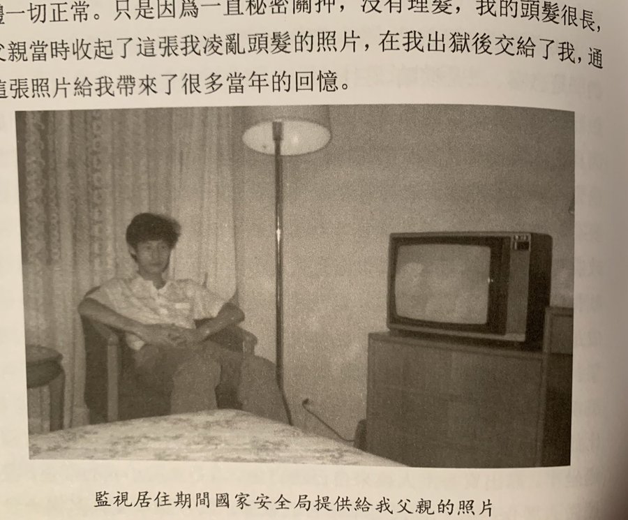
在1988年,我在北大等地发起“民主沙龙”,公安部常务副部长亲自挂帅了一个专门监督我的工作组,对我软硬兼施,甚至讲卧底父亲请到北京,就是要招安我成为第三梯队,还承诺给送发双份工资,声称:
刘刚在北京,公安部没法保证北京的安定团结。
就在这个节骨眼上,俞雷部长又派人找到我。我拒绝接见俞部长。与部长就将我当警察的父亲接到北京。我父亲也是拒绝俞部长的请求,俞部长就说这是公安部给我父亲安排的特殊工作,实际上就是特务工作吧。我父亲就不得不来到北京。@riverqu @chinashiyu @KwokMiles
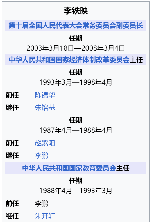
1994年,我被关押在凌源第二监狱。就是我在监狱期间,中国也对我是念念不忘,几次派高官去监狱里招安我。这次派的是当时的国务院新闻办主任(当前的人大法工委主任)曾建徽。曾建徽号称是中共的笔杆子兼法学师爷,当年的4-26社论及《中国的人权状况白皮书》都是他的亲笔大作。
高智晟,顾晓军,和杀鸡儆猴
http://jasmine-action.blogspot.com/2016/07/blog-post_9.html
照片上的这位叫曾建徽,94年时是国务院新闻办主任。他曾经带上百号人专程从北京前往凌源监狱去探视我,同我进行谈判。
新闻办主任曾建徽率中外记者到监狱探访刘刚的故事
原文网址:http://jasmine-action.blogspot.com/2022/05/blog-post_67.html
推特链接:
就凭下面的这几件事,就可以证明中共政权罪了解刘刚在1986年之后的中国历次民主中的核心作用:
【1】1993年8月,中国政府派新华社、中国日报、北京周报、人民日报海外版等英文媒体的记者前往凌源第二监狱采访刘刚,并在国外作了长时间的污名化报道。
1994年,我被关押在凌源第二监狱。就是我在监狱期间,中国也对我是念念不忘,几次派高官去监狱里招安我。这次派的是当时的国务院新闻办主任(当前的人大法工委主任)曾建徽。曾建徽号称是中共的笔杆子兼法学师爷,当年的4-26社论及《中国的人权状况白皮书》都是他的亲笔大作。
高智晟,顾晓军,和杀鸡儆猴
照片上的这位叫曾建徽,94年时是国务院新闻办主任。他曾经带上百号人专程从北京前往凌源监狱去探视我,同我进行谈判。
中国有外事办主任去监狱探视过其他政治犯吗?
新闻办主任曾建徽率中外记者到监狱探访刘刚的故事
推特链接:
就凭下面的这几件事,就可以证明中共政权罪了解刘刚在1986年之后的中国历次民主中的核心作用:
【1】1993年8月,中国政府派新华社、中国日报、北京周报、人民日报海外版等英文媒体的记者前往凌源第二监狱采访刘刚,并在国外作了长时间的污名化报道。
刘刚
2024年2月14日


 : An economic system that contains some sub systems. It can be as small as a family, a firm, and can be as large as a country or the whole world.
  is also called a macro system compared with its sub systems.
 : An integer represents the total number of the sub systems in
  .
. : An integer represents the total number of the products that are produced in
  .
. : The ith unit or sub system in system
  . It could be an individual member, or a group of people, such as a firm or another economic system in
  . However, there are no overlaps between different Units. For example, if an individual has been included in one unit, the same individual can’t be included in another unit.
  is also called a micro system compared with its parent system.
 : The kth product that can be produced in system
  . Actually, the product here means any labor activities that can be done by any unit in
  . It can be a real product, a project, a job, a task, and anything that need to be done or produced by any unit in
  .
. : A time span that the above mentioned products are produced in
  .
. :
:  , which is the set of non-negative M-dimensional real vectors and with the original point
  excluded.
 : The same as
  . However, we use it to particularly represent the Production Space with its kth Cartesian coordinate representing the amount of a parameter related to
  product.
 : The demand amount of
  product that requested by
  .
. : The maximum amount of
  product that can be produced by
  within time
  . Normally
  can be produced by
  when it uses all of its resources to work on product
  . All the
  make up an
  matrix, which is called the micro capability matrix of system
  .
. : The amount of
  product that are actually produced by
  . All the
  make up a vector in
  , and is called micro supply vector.
 : The amount of
  product produced by the macro system
  . It is also called the macro supply of system
  . All the
  make up a vector in
  , and is called a macro supply vector of system
  .
. ;
;  : The price of the
  product in system
  .
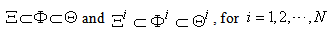
. introduced above. An economic system is called a micro system if it is contained in a macro system, such as the sub-system
  described above.Definition: System Parameter: An economic parameter is called a system parameter if it is associated with an economic system. For example, the supply amount, demand amount, and price are all examples of system parameters.Definition: Micro Parameter and Macro Parameter: A system parameter is called a micro parameter if it is associated with a micro system, and is called a macro parameter if it is associated with a macro system. Some parameters may be associated with both micro system and macro system. As long as there is no confusion, we use the same alphabet character to represent a system parameter: if
  denotes a macro parameter associated with a macro system
  , then
  will be used to denote the same micro parameter associated with micro system
  .For example,
  and
and  represent the macro and micro supply amounts of product
  ,
,  and
and  denote the macro PPF of system
  and the micro PPF of the micro system
  correspondingly.Definition: Vector Parameter and Scalar Parameter: a system parameter may also be associated with each of the production, for example, supply amount normally means the amount of a product that can be provided by an economic system. In a system with
  products, a system parameter could be
  -dimensional with each component representing the amount associated with one product. These
  -dimensional parameters make up a vector in the production space
  , thus is called a Vector Parameter. A vector parameter can be represented by a vector in
  . Examples of vector parameters are: Supply, Demand, and Price.A system parameter is called a scalar parameter if it is one dimensional. Examples of scalar parameters are: income, GDP, revenue, etc.Additive Parameter: A system parameter is called additive parameter if the corresponding macro parameter can be derived by aggregating the same parameter over all of its micro systems. Or precisely, system parameter X is additive if
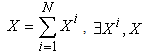
 is a parameter reachable and meaningful to micro system
  , while
  is the same parameter reachable and meaningful to macro system
  .In our model, we tried to decompose the macro system
  into some micro systems
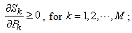
  , and divide the products into some products or tasks in such a way that some of the system parameters are additive, particularly, the supply amount, the demand amount, revenue, and income are all additive. However, the price parameter is not an additive parameter.Based on the above notations and definitions, we can say that the supply and demand are vector parameters and are additive, whereas the price is also a vector parameter, but not additive. The income, revenue, GDP, profit and loss are all additive scalar parameters. We are only interested in those parameters in this paper.
 , the production capability matrix for each micro system and for each product.
 : The macro demand of
  product that needs to be accomplished by system
  .We assume the following parameters are unknowns and need to be resolved: Price, micro supply, macro supply, micro income, macro revenue.
 , let us assume that it can arrange its resources to make any requested products. However, its production amount for product
  should be limited to or bounded by
  due to its limited resources and capabilities. Any of its feasible production state will be a point or a vector in the production space
  . All of its feasible production vectors should be a bounded range in the production space
  . We call this bounded range as its micro Production Possibility Range (PPR) and denoted as
  . The upper boundary of
  is called the micro PPF, denoted as
  . Normally, as long as the micro system
  is small enough compared with macro system
  , each of the micro PPF can be approximated by the linear plane curve that passing the
  axis at
  in production space
  .Given the micro capability matrix, the micro PPF
  can be formulated as:
 can also be expressed in the following format:
 is called the intrinsic price vector of the micro system.Actually,
  is a linear plane curve with vector
  as its normal vector. It passes the
  axis at the points:
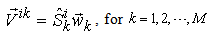
 is the unit vector on the
  axis.
axis.  and is on the
  axis of the production space. We call these
  points as the micro vertex points.Given the price vector as
  and the micro supply vector
  of the micro system
  , the total income or revenue of the micro system
  can be expressed as:
 is feasible to micro system
  , there should have some possible micro supply vectors that can maximize the income or revenue of the micro system
  . Such feasible micro supply vectors can be formulated as:
 to be maximized is a linear function, according to Lagrange’s theorem, the max-min can only be found on the boundary of the region
  . Then the above equation is equivalent to:
 vertex points listed in Equation (5). Then, the above equation can be further simplified as:
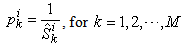
 is an
is an  function defined as:
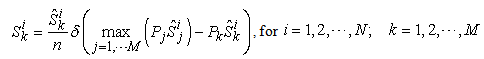
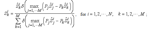
 is the total number of vertex points that have
  maximized for
  . Number
  can be formulated as:
 maximized. It gives at least one of the micro supply vectors
  that can have the micro income
  maximized. It is an explicit mathematical format for the micro supply as a function of the capability matrix and the price vector. However, it is a discrete function and thus is difficult to deal with. The key step and major contribution of our model is to formulate a continuous and smooth function to approximate the Equation (13). Here are the key steps. Equation (13) is equivalent to the following function:
 is called the macro capability parameter defined as:
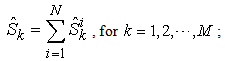
 .In practical applications, we can simply drop the limited function by assigning
  with a large number, thus the Equation (14) can be simply expressed as:
 for
for  ;Normally, it will be good enough if we assign
  as:
as: Equation (16) will be a good approximation for the micro supply function, and it gives the Micro PPF
  once the price vector goes through all possible directions in the production space
  .
.  will be good enough for most of the practical applications. We use
  to get most of the results listed in this paper.
 and the micro supply as a function of the price vector and the capability parameters, as shown in Equation (16). As each of the micro system
  has a maximum production frontier and a limited range as its PPR, the macro system should also have a macro PPR in the production space
  , and must have a macro PPF. As the supply parameter is an additive parameter, we can get the macro supply vector by aggregating all the micro supply vectors, that is:
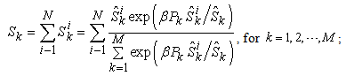
 , as shown in Figure 3. So, the above Equation is not only a supply function, but also a function that gives the macro PPF
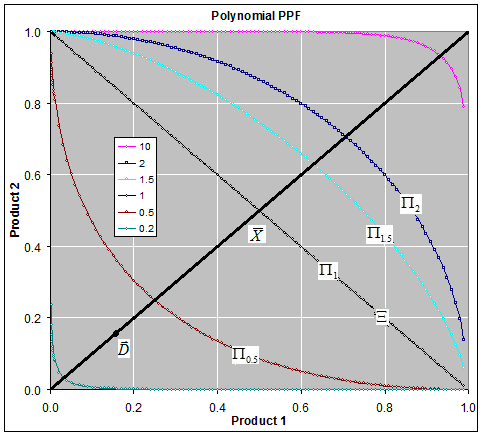
  .Figure 4.shows the Supply-Price curves for various
  values. Once
  is big enough, the Supply-Price curves become step curves. Keeping in mind that each micro system is targeting at maximizing its income, so, when the price
  rises, a micro system
  may want to switch all of its resources to work on product
  , and thus to have the macro supply
  be suddenly increased by an amount of
  . At the same time, because
  switched from working on
  to work on some other products, such as
  (
( ), it will have the supply
  decreased suddenly by an amount of
  . This explains why the Supply-Price curve shows as a step curve, also explained the Law of Supply as discussed in later sections.The supply functions and the PPF given in Equation (17) are the key contributions of this paper. The rest of the paper discusses applications of this supply function, or compare our PPF with some other production possibility frontiers and see how much efficiency can be improved by using our proposed model.
 denote the micro WPPF of micro system
  , and
, and  denote the macro WPPF of the macro system
  .
.  is defined as the lower boundary under the conditions that all of its micro systems have reached their micro PPF
  . The WPPF
  is defined as the set of micro supply vectors that are on the
  and results a macro supply vector on the macro WPPF
  if aggregated for all micro systems.
 and
and  can be formulated using the same Equations as shown in Equation (16) and (17), as long as we set
  . We will not rewrite these Equations here.Let
  be the region bounded by
  and
and  , and
, and  be the region bounded by
  and
and  .
.  is called the micro Maximum Production Possibility Range (MPPR), and
  is called the macro MPPR.Given a price vector
  , through Equations (16) and (17),we can get a macro supply vector
  on
on  , a macro supply vector
  on
on  , a micro supply vector
  on
on  , and a micro supply vector
  on
on  . It can be shown that the price vector
  is the normal vector of those curves at the corresponding points as indicated by these supply vectors [6].
 denote the supply elasticity for the
  product. By applying partial differentiation to Equation (16) and (17), we can easily have:
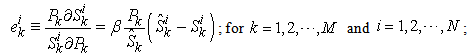
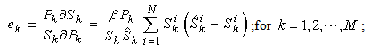
 given in Equation (19) is non-negative. Noting that
  and
and  , thus all items in Equation (19) is non-negative, then the elasticity
  which is a sum of some non-negative numbers is also non-negative. Thus Equation (20) is proven.By applying partial differentiation to Equation (16), we have:
 ,
, ,for
,for  and
and  Equation (21) follows the above two equations immediately, and thus the Law of Supply is proven.
 and
and  are functions of
  . Thus, the above general equilibrium equation gives
  equations with
  prices as unknowns. Generally, once we know the function format for
  and
and  , the equilibrium price vector can be solved from Equation(22).We do not try to give a generic format for demand functions in this paper, instead, we just simply assume the demand is given as a vector with fixed direction, thus Equation (22) can be expressed as:
 equations with
  for
for  as the
  variables. Then the price victor
  can be solved by solving the above equation through many mature methods, such as Newton’s method [5, 9], Brent’s method [2, 13]. Thus all the micro supplies
  can be given through Equation (16), and all the macro supplies can be given through Equation (23) or Equation (17).
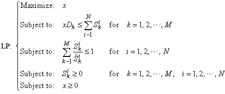
 and
and  as variables. It can be easily solved through the T-forward method [7, 8, 3]. Equation (24) and (25) should give the same solution.
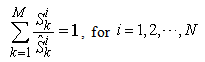
 . Similarly, we can construct a macro LPPF curve
  for the macro system
  , which can be formulated as:
 and
and  be the micro SPPF and macro SPPF for the Self Sufficient scenario.
  is the same as the plane curve
  as shown in Equation (26). However, the macro SPPF
  is different from the Macro LPPF
  .By definition, given the requested demand as
  , the micro SPPF
  can be expressed as:
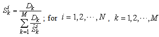
 can be formulated as:
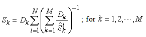
 is called the carpenter system, which contains
  units or members, and need to make
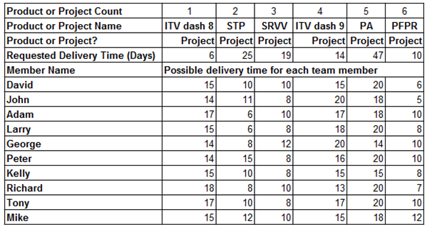
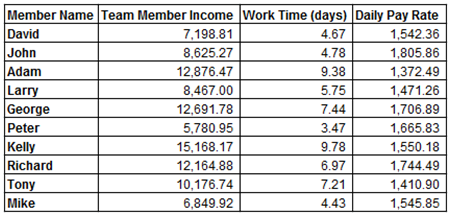
  products. The carpenter system needs to produce 4 table legs, 1 table top, and 6 chairs, which make up the 3 components of the demand vector. The micro capability matrix and demand vector are listed in Table 1. The requested amounts or demands are listed in row 3, and the production capabilities are listed in row 5 to 14.
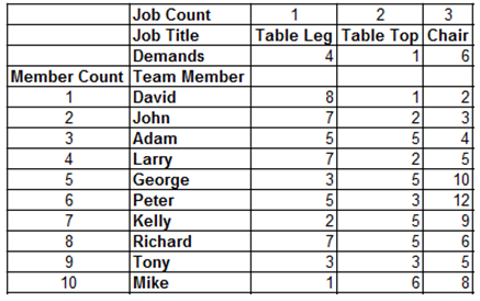
 ,
,  ,
,  , and
, and  are derived and are drawn in Figure 2. These four curves are all converged to the same plane curve.
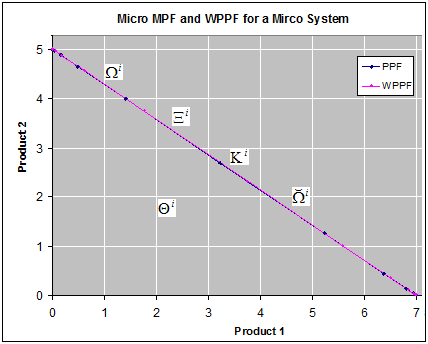
 , the micro WPPF
  , the micro LPPF
  , and the Micro SPPF
  are all shown as the same plane curve in the production space
 and
and  could be different from the plane curve for some small
  . However, the difference can be only shown up for 3 or more dimensional case. If we set all other prices to 0 except two of them, then the above four curves always converge to the plane curve.Figure 3. shows the macro PPF
  , along with some other macro curves, including WPPF
  , LPPF
  , and SPPF
  . Figure 4 draws the supply-price curves for various
  value. By comparing with Figure 1, our model gives the PPF and supply functions in more detailed formats and make the general supply-demand equilibrium solvable numerically.
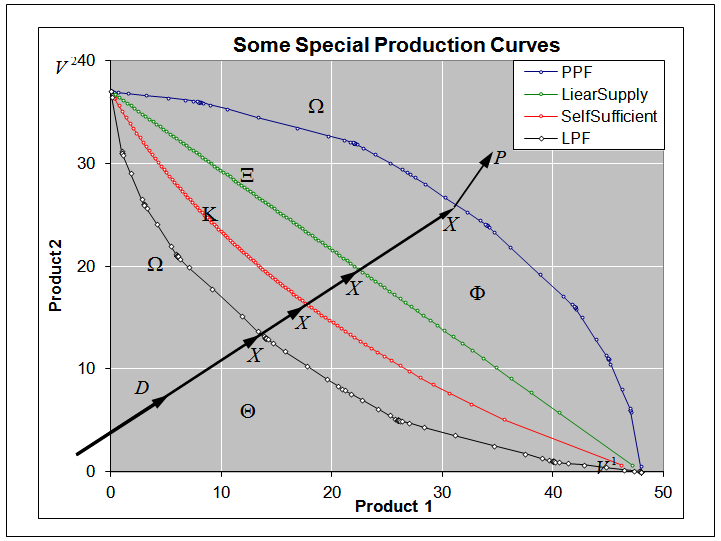
 is a convex curve, the macro WPPF
  and the macro SPPF
  are concave curves, whereas the macro LPPF
  is a linear plane curve in the production space. The maximum PPR
  is the region bounded by
  and
and  . The extension line of the demand vector
  intersects with these 4 curves at the points
  ,
,  ,
,  , and
, and  respectively. These curves and points are used for improved efficiency analysis
 has reached its micro PPF
 , then the aggregated macro state of the macro system must be in the macro MPPR
 . Also, suppose the macro system
  is requested to produce the demand vector
 . The demand vector
  is as shown as the line
  in Figure 3. Figure 3. also shows the four points
 ,
,  ,
,  , and
, and , which are the intersection points of the line
  with the curves
 ,
,  ,
,  , and
, and .For all possible production states in
 , the Line
  gives all possible states that are proportional to the requested demand
 . Any other states in
  may have some products wasted or not needed compared with the requested demand
 . So, for all possible states in
 , only the states on line
  can best meet the requested demand
 . We are only interested in the states that are on the line
 .For all states on the line
 , the point
  is the best scenario, because it gives the maximum possible amount for all supplies,
  is the worst scenario, whereas
  and
and  are somewhere in the middle. Point
  can be treated as the average state for all points in the macro MPPR
 .Let us assume that point
  is the average state that the macro system reached without using any optimal management method. Now, let
  denote the improved production efficiency by comparing the best scenario
  with the average scenario
 , then
  can be formulated as:
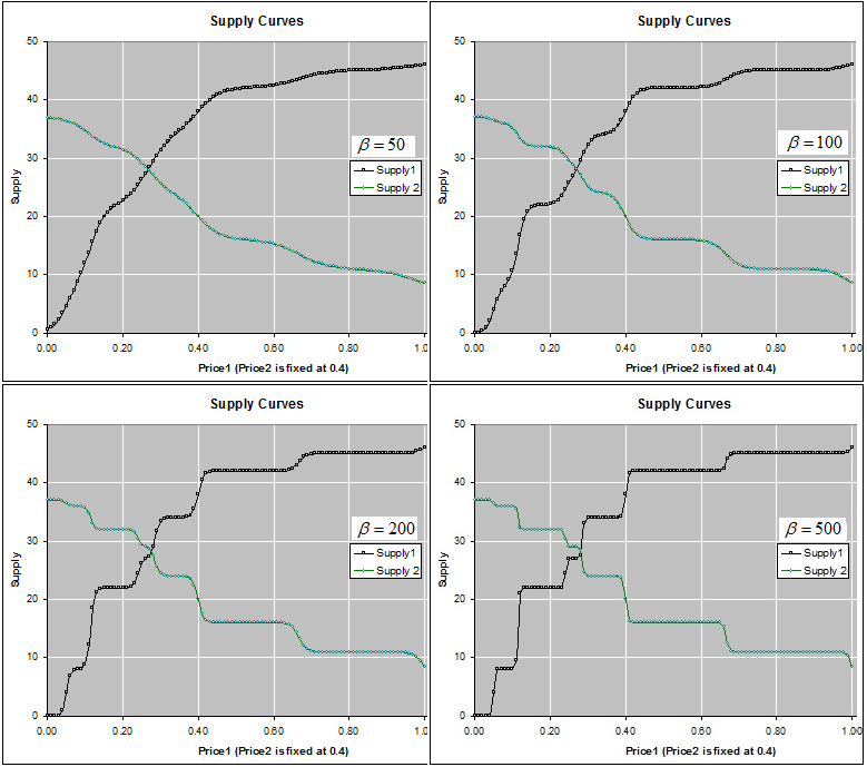
 rises and all other prices remain unchanged, the supply
  rises, whereas the supply for other products decreases, for example, Supply
  decreases. When
  is large, the supply curves
  and
and  become step curves
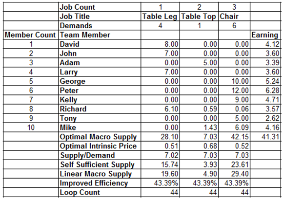
 and proportional to the requested production demand vector
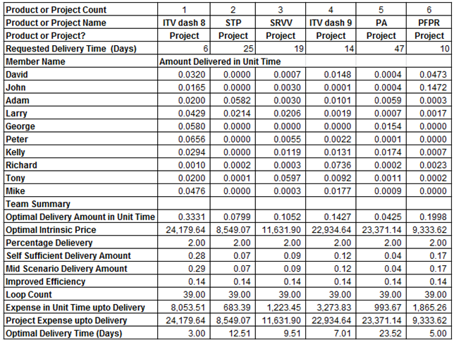
  .The last column gives the Earnings or Incomes for each team member.The row with header “Supply/Demand” gives the number
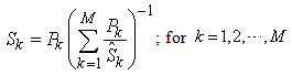
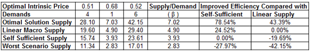
 defined in Equation (23). It is the ratio between the optimal solution and the requested demand amount.The row with header “Optimal Intrinsic Price” gives the intrinsic prices which can be used to calculate the earnings for each team member. The intrinsic price vector for these 3 products should be (0.51, 0.68, 0.52). Once this intrinsic price vector is known, each team member will reach his maximum income by making the products with the amounts as requested in the optimal solution. In other words, the whole team will realize the optimal solution automatically as long as each sub unit has maximized its income.The row with header “Self Sufficient Supply” lists the supply state
  on the SPPF
  .The row with header “Linear Macro Supply” lists the supply state
  on the LPPF
  .The row with header “Improved Efficiency” lists the improved efficiency ratio by the optimal solution
  compared with the Linear Macro Scenario
 .The row with header “Loop Count” lists the number of loops for our numerical calculation to converge to the results with required precision.The optimal solution not only depends on the capability matrix, but also depends on the direction of the demand vector. Given a team member and his capability matrix, we cannot tell which product is the most specialized product for him. The optimal solution may request him to work on one product. However, once the direction of the demand vector changes, the same team member might be requested to work on some other products to have the whole team to reach the optimal solution.
 can be explained as the delivery ratio (or amount) of the kth project
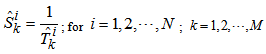
  by team member
  . The demand for each project is 1 within required delivery time.Let
  denote the required delivery time for the kth project
  , and
, and  denote the fastest delivery time of team member
  to deliver the kth project
  under the condition that
  works only on project
  . Then the equivalent demand vector can be expressed as:
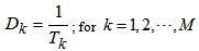
 , we can find the improved efficiency ratio by the optimal solution. The improved efficiency for the carpenter team is:
 in this section. Let
  be the intersection point of the demand vector
  (or its extension) with the curve
  , and
, and  denote the length of the line
  . Then
  can be easily found as:
 is a convex curve, we can use
  to approximate the PPF
  , with
  to be a value that can make the
  most close to
  . Normally, once we find one point on
  , we can calculate the value of
  which can make the
  most close to the
  . Further, we assume the average production state is roughly at the point
  on the curve
  (or denoted as
 ). If
). If  is used to approximate
  , the improved efficiency by reaching the macro PPF can be estimated as:
 is a good approximation for
  when
when ; and even
  will be a good approximation for
  when
when  and
and .To make it more conservative, we use
  to approximate the macro PPF
 . Then the production efficiency ratio that can be improved by the optimal solution can be estimated as:
 products.Based on our test results and the above analysis, our optimal solution for team work management normally can improve the production efficiency by 40% for most of team work problems!
 can be used to approximate the PPF
  and LPPF
  . Here all the curves are shown in 2-dimensional. You need to imagine it in M-dimensional
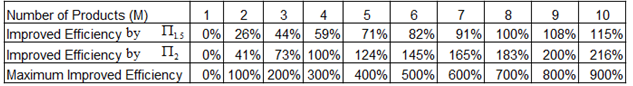
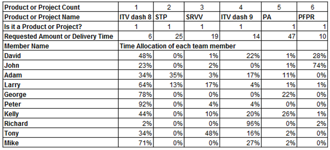
 , and the micro income amount
  . Using these micro information, a team manager can tell each team member
  to work on the
  with the amount
  as indicated in the optimal solution. Note that most of the team members may work on only one product. The team manager can also tell each team member
  about how much he should be paid, which would be
  . So, with micro management, a team manager manages each of the team members in micro details, including what and how much need to be done, as well as how much should be paid as return. That is why we call this management method as Micro Management.
 . Given this intrinsic price vector, each team member will reach his maximum income by working on the product with the amount as requested by the optimal solution. Suppose each team member is targeting at maximizing his income, the team manager needs only declare the intrinsic prices, then, every team member will automatically to work on the product with the amount such that the whole team will reach its optimal solution as indicated in the optimal solution.The team manager doesn’t manage the team members in micro details, but manage it in macro level, which simply tells how much will be paid for product or project to be delivered. That is why we call this management method as macro management.